Motivation
My father showed me this square when I was eight or nine.
It made such a strong impression on me that I memorized it and took every opportunity to show it off. Some years later, I discovered in a book my math teacher gave me that those squares were called “magic squares” and came in various sizes (except 2 and 6). In a magic square, numbers from to are arranged in an grid such that the sum of each row, column, and both main diagonals is the same constant. This topic was the obvious choice for one of the first computer programs I wrote: a program that generates and draws magic squares.

Melencolia I (1514) by Albrecht Dürer, featuring a magic square in the upper right corner. Source: wikipedia
Magic squares have fascinated people across cultures and eras. Many renowned mathematicians, including my favorite one, Leonhard Euler, have enjoyed studying them. Magic squares have also been attributed mystical, divinatory, and symbolic meanings.
I am not superstitious, but when I read that Ernő Rubik initially called the most iconic toy in history Bűvös Kocka (the Magic Cube), I took it as a sign from the universe. I read this sign as an invitation to close the loop by adding an extra dimension to the program that I wrote as a young person and investigating how to programmatically solve the Rubik’s Cube.
Introduction
This is my travel diary through the Land of the Cube. It started a few months ago when my father-in-law gave us a 2x2 Rubik’s Cube. Then I read Cubed (Weidenfeld & Nicolson, 2020), an intimate account by the otherwise introverted and reclusive Ernő Rubik. I then started researching, gaining intuition, and finally coding various algorithms to solve the cube. Besides being an iconic symbol of pop culture, the cube has left a profound mark on the history of mathematics and computer science. Several classic search algorithms that I will cover here were developed in relation to it.
This accompanying repository contains a collection of algorithms for solving the cube, ranging from elementary algorithms that are simple to understand but potentially intractable, such as BFS and IDDFS, to more tractable algorithms that still might require more memory than a modern (2025) laptop has. Finally, there is a completely different category of algorithms based on group theory. The pinnacle of these algorithms is Kociemba’s two-phase algorithm, which exploits the cube’s symmetries, and uses with precomputed heuristic tables.
To gain intuition and avoid the combinatorial explosion that comes with the 3x3 cube, I will start with the smallest of all: a 2x2 cube. I will progress from simple, classic algorithms to more complex, specialized, and efficient ones.
Notation
How would you represent a cube? I’m probably not alone in coming up with a representation that essentially opens the cube into a 2D shape, like this:
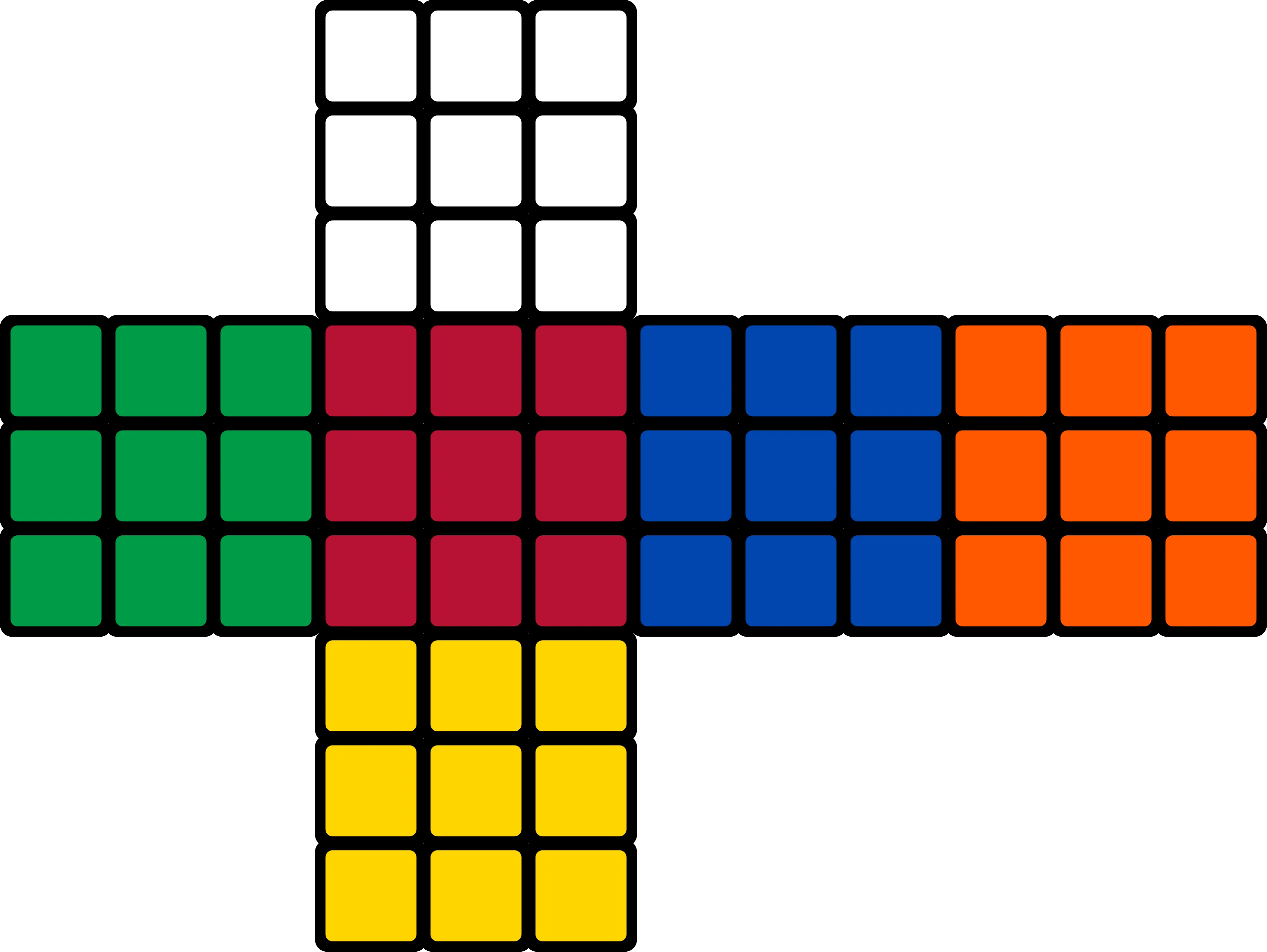
Source : wikipedia
So, my original cube representation is a numpy array.
I adopted the following notation for moves, where each face can be turned 90 degrees clockwise (), 90 degrees counterclockwise (), or 180 degrees (), where . For example, moving the upper face 90 degrees clockwise is denoted as . Moving it 90 degrees counterclockwise is denoted (in alternative notations, it is or ), and moving it 180 degrees is denoted (in alternative notations, it is ). In general, , , , are quarter metric clockwise turns, their inverses are for instance . The inverse of a sequence like is .
First approach: uninformed search
When discussing Rush Hour with my colleagues, I showed them the following table:
| Algorithm | Complete | Optimally efficient | Cost-optimal |
|---|---|---|---|
| DFS | ❌ | ❌ | ❌ |
| BFS | ✅ | ❌ | ⁉️ |
| ✅ | ✅ | ✅ |
This table lacks two important dimensions that are irrelevant in the Rush Hour case and in many every day problems but will be important in the Rubik’s Cube case: time and space complexity.
According to the Book 📗, despite its many (apparent) disadavantages, DSF is the workhorse of many areas of AI because of its low memory requirements. BFS has a very scary quadratic space complexity.
Nevertheless, let’s start with BFS to illustrate the problem. I started with a 2x2 cube.
The 2x2 cube has possible configurations, resulting from 8 corner cubies that can be permuted in ways, and each cubie can be oriented in 3 different ways. After discounting 24 symmetries, we are left with:
If the 2x2 cube is correctly fixed to avoid counting symmetries —for example by fixing the corner and allowing only , , and moves— then we will visit at most e states, which is easily maneageable with BFS, even without memory optimizations.
In cube-related computer science literature Richard Korf’s name often comes up. He implemented one of the first optimal solvers and developed several of the algorithms that are commonplace today, including IDDFS (Iterative Deepening Depth First Search) and (Iterative Deepening ).
IDDFS is the next step. It provides a more memory-efficient alternative to BFS while retaining all of its beneficial properties.
def iddfs(start_state, goal_state, max_depth):
    for depth in range(max_depth):
        result = dfs(start_state, goal_state, max_depth=depth)
        if result is not None:
            return result
    return None
Code box: Basic structure of IDDFS
Both BFS and IDDFS can solve 2x2 cubes without issue. They can also solve 3x3 cubes that are close to the solved state (i.e., that are not very scrambled). However, they become intractable for very scrambled 3x3 cubes.
The 3x3 cube is a different beast
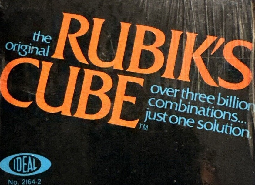
Figure: Box of the original Rubik’s Cube distributed by Ideal Toys
When Ideal Toys first marketed the cube, the advertised it as having over three billion combinations. They were a bit off.
Ideal Toy Company stated on the package of the original Rubik cube that there were more than three billion possible states the cube could attain. It’s analogous to MacDonald’s proudly announcing that they’ve sold more than 120 hamburgers.
J. A. Paulos, Innumeracy
The actual number is over 43 quintillion. 8 corners that can be arranged in ways, each with 3 orientations, and 12 edges that can be arranged in ways, each with 2 orientations. Discounting 24 symmetries, we get:
This number is approximately . If we manage to visit states per second, and that’s ambitious in Python, it would take:
That’s not the age of the universe, but is still quite a wait. Right? And that’s without considering memory limitations.
Meet in the middle
One difference between the cube case and Rush Hour is that we know the goal state in the cube case. This knowledge can be used to reduce the search space. Using bidirectional search, we can search from both the initial and goal states simultaneously until the two searches “meet in the middle.”
This replaces a search space of size with two search spaces of size each. The total number of states visited is then , which is instead of in the 3x3 cube case.
A few years ago I saw a very nice report by two students at ETH who claimed that their C implementation of meet in the middle required about 90 GB of RAM and 4 hours to solve a random cube.
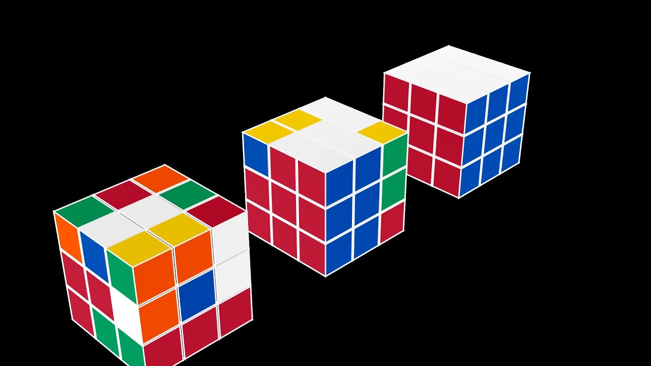
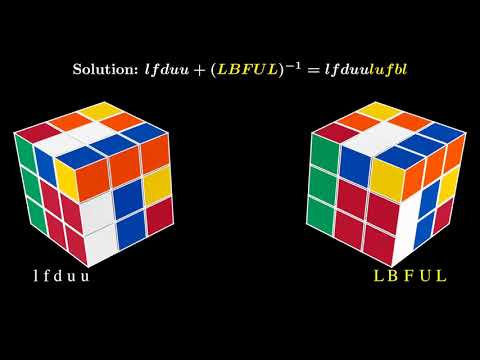 A video generated by my implementation of meet in the middle
In the previous video, the solutions found by the front and back searches are: and respectively. To obtain the full solution, we must reconstruct the path. It would be + = + = + = .
If you are familiar with matrix algebra, you might recall that the inverse of a product is also . This is true for any group and is intuitive when you think about putting on your socks and shoes. The inverse operation is first removing the shoes and then the socks .
Although not related, this brings us to the next topic, where the beauty and generality of group theory will be exploited to achieve a very elegant and efficient algorithm.
Kociemba’s two-phase algorithm
A video of a solution found by Kociemba’s two-phase algorithm
The basic idea is that the cube can be described at the “cubie” level.
The cube is made up of 27 smaller cubes, 26 of which are visible. These small cubes are called “cubies”. Like quarks, cubies come in different flavors:
- Face or center cubies: the ones at the center of each face (they have one color)
- Edge cubies: the ones showing two faces (two colors)
- Corner cubies: the 8 cubies at the corners of the cube, each showing 3 colors.
In this new cube representation we keep track of corner cubies and edge cubies. Any valid position of the cube can be described by the permutation and orientation of these cubies.
We can then define a group, , of all possible cube permutations (the group of all permutations of a set is called the symmetric group). More specifically, it is defined as , where the operation , multiplication, is the composition of sequences of moves. Each sequence of moves has an inverse , and the identify operation is to do nothing to the cube.
The author does a good job in describing his algorithm so I will not repeat his description here. I will just explain the concepts that I found the most interesting.
As in many other areas of mathematics and the natural world, one of the most important concepts is counting. In this case, counting the permutations of the cube is critical. The algorithm uses with precomputed heuristics. These heuristics measure the distance from any given position to the desired goal position. It is important that the heuristics are admissible; that is, they should not overestimate the distance to the goal. To efficiently store and retrieve these heuristics, the algorithm counts permutations using a Lehmer code (or a variation of it), as well as binomial coefficients, to uniquely map each permutation to an integer in a compact way. These integers serve as keys in the precomputed heuristic tables (pattern databases), and the corresponding values represent distances modulo 3. There is an ambiguity that can be resolved later in the search. Pruning tables are generated with BFS from the goal state.
Kociemba’s algorithm is based on Thistlethwaite’s algorithm, which also uses group theory and cube symmetries to reduce the search space in four phases. However, Kociemba’s algorithm uses only two phases.
Phase 1, reduction to subgroup
The goal of this phase is to reach a state in which the cube can be solved using only moves. . By the end of this state, all corners and edges will be correctly oriented, meaning the corner cubies will not be twisted and edge cubies will not be flipped. All slice edges (the 4 UD-slices edges) (FR, FL, BL, and BR) will be in the middle layer. This phase uses three operations: twist (0 - 2186), flip (0-2047), and slice (0 - 494). Phase 1’s problem space has different states. See the code for more details. This part of the algorithm uses (Iterative Deepening ), which is to what IDDFS is to DFS. The same heuristic is used, but the pruning threshold for is adapted. It was developed by Korf and is one of the most widely used algorithms for problems that cannot fit in memory.
- Constraints: All 18 face moves are allowed, i.e., , , for .
Phase 2: solving from subgroup to the solved state
The goal of this phase is to restore the cube to the solved state using only moves generated by the subgroup . During this phase, the corners and edges are permuted into their correct positions. This phase uses three operations: corners (0 - 40319), ud_edges (0 - 40319), and slice_sorted (0 - 23). This phase also uses . Phase 2’s problem space has different states. See the code for more details.
- Constraints: Only moves preserving are allowed, i.e., moves generated by , which also includes inverses and double turns of and . However, moves like and are excluded because they cannot be generated by this subgroup.
Kociemba’s algorithm exploits the cube’s symmetries to reduce the search space even further, although this is not required for the algorithm to work. The code generates 48 symmetries with these operations:
ROT_URF3: 120° rotation around a diagonal.ROT_F2: 180° rotation around the F-B axis.ROT_U4: 90° rotation around the U-D axis.MIRR_LR2: Reflection.
Final thoughts
Abstract algebra is a beautiful subject. It provides a general framework for studying structures that appear in many areas of mathematics and science. Rubik’s Cube is a prime example. I plan to write a follow-up post that delves deeper into the concepts I reviewed, but there are already excellent sources on the subject. This is a superb one: Group Theory via Rubi’s Cube.
Working on puzzles is a delight I recently discovered. It is really engaging and stimulating. In a deeper sense, it is also a reminder that it’s important to keep learning and challenging oneself without utilitarian goals in mind. But let’s not forget the most important aspect: fun. After all, we are Homo Ludens.
Finally, many things I read in Cubed resonated with me, like the idea of embracing a problem and following through with it until it is solved or a better, more interesting problem is found.
References
- Cubed (Weidenfeld & Nicolson, 2020), by Ernő Rubik
- Artificial Intelligence: A Modern Approach (4th Edition, Pearson, 2020), by Stuart Russell and Peter Norvig.
- https://kociemba.org/
- https://cube20.org/
- https://tomas.rokicki.com/rubik20.pdf
- http://www.geometer.org/rubik/
- https://web.mit.edu/sp.268/www/rubik.pdf
- https://www.fuw.edu.pl/~konieczn/RubikCube.pdf